This notebooks demonstrates iterations and recursions in EMT.
Our first example is the growth of an amount of money at an interest rate of 5%.
>q=1.05; iterate("x*q",1000,n=10)'
         1000
         1050
       1102.5
      1157.63
      1215.51
      1276.28
       1340.1
       1407.1
      1477.46
      1551.33
      1628.89
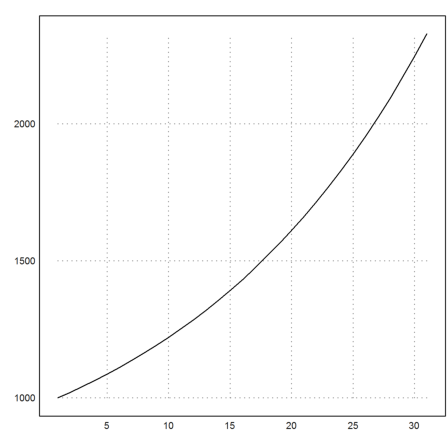
Let us subtract the amount of 30 in each year, while adding interests, and plot the result for 30 years.
>plot2d(iterate("x*q-30",1000,n=30)):
As always in EMT, we could also use a function and call collection to pass additional parameters (or, alternatively, semicolon parameters).
>function addf(x,q,a) := round(x*q+a,2); ...
 iterate({{"addf",1.05,30}},1000,n=6)
[1000, 1080, 1164, 1252.2, 1344.81, 1442.05, 1544.15]
Iterating like this is a simple form of recursion,
![]()
For more complicate sequences, we use the function "sequence". This function computes the value x[n] from all previous values x[1],...,x[n-1] given in a vector. Additionally the variable n can be used.
Here is an example computing the Fibonacci numbers.
![]()
>sequence("x[n-1]+x[n-2]",[1,1],10)
[1, 1, 2, 3, 5, 8, 13, 21, 34, 55]
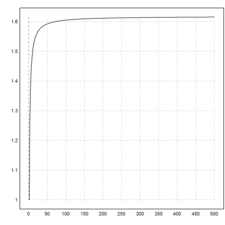
The n-th root of the Fibonacci numbers converges to the golden ratio.
>plot2d(sequence("x[n-1]+x[n-2]",[1,1],500)^(1/(1:500))):
Clearly the same can be done with a loop, either inside a function or in a multi-line.
>x=ones(500); for k=3 to 500; x[k]=x[k-1]+x[k-2]; end;
We can compute recursions which depend on all previous elements. In the following example, the n-th element is the sum of all previous elements. This time, we start with a scalar value 1. Of course, the result is 2^n.
>sequence("sum(x)",1,10)
[1, 1, 2, 4, 8, 16, 32, 64, 128, 256]
Instead of an expression in x and n, we can also use a function.
In the following example, we iterate
![]()
where A is a Matrix, and each x[n] is a 2x1 vector.
>A=[1,1;1,2]; function step(x,n) := A.x[,n-1]
>sequence("step",[1;1],5)
            1             2             5            13            34
            1             3             8            21            55
There is the function "matrixpower" which yields the same result. This function is faster, since it uses only log_2(n) matrix multiplications.
>matrixpower(A,4).[1;1]
           34
           55
Of course, we could also use a loop in a function, or in the command line.
>x=[1;1]; loop 1 to 4; x=A.x; end; x,
           34
           55
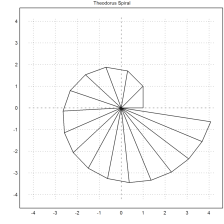
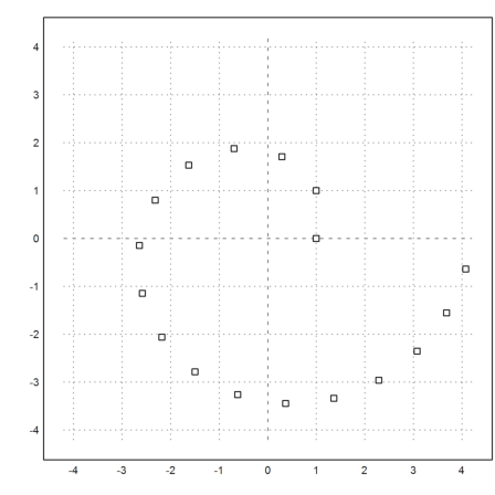
As an example, we produce the spiral of Theodorus recursively. The recursion is
![]()
which produces a series of complex numbers. See
>function g(n) := 1+I/sqrt(n)
Now we can run the recursion and get a sequence of 17 complex numbers.
>x=sequence("g(n-1)*x[n-1]",1,17); plot2d(x,r=4.2);
We add the connections from 0 to the points in a loop.
>for i=1:cols(x); plot2d([0,x[i]],>add); end; ...
   title("Theodorus Spiral"):
If you look at the definition of this curve, you see that you can also use a recursion, which does not use the index n.
And, of course, we do not have to use complex numbers. Instead we use column vectors in the plane.
>function gstep (v) ...
 w=[-v[2];v[1]];
 return v+w/norm(w);
 endfunction
If we iterate 16 times starting from [1;0], we get matrix with the columns containing our vectors.
>x=iterate("gstep",[1;0],16); plot2d(x[1],x[2],r=4.2,>points):
Often, we want to iterate until convergence. If the function does not converge, the user has to press the escape key to stop the iteration!
>iterate("cos(x)",1)
0.739085133216
If such an iteration converges, the limit is a solution of
![]()
This examples does also work with interval arithmetic.
>res := iterate("cos(x)",~1,2~)
~0.739085133211,0.7390851332133~
If we make res a little larger, we are able to prove that h contains a fixed point of cos.
>h=expand(res,100), cos(h) << h
~0.73908513309,0.73908513333~
1
Or we could set up a function for the iteration.
>function f(x) := (x+2/x)/2
The iteration x(n+1)=f(x(n)) converges quickly to sqrt(2).
>iterate("f",2)
1.41421356237
It might be easier to use an expression in x instead of a function.
>iterate("(x+2/x)/2",2)
1.41421356237
The function "iterate" with the parameter "n=..." returns the history of 5 iterations.
>iterate("f",2,5)
[2, 1.5, 1.41667, 1.41422, 1.41421, 1.41421]
Starting with an interval does not work.
>niterate("f",~1,2~,5)
[ ~1,2~, ~1,2~, ~1,2~, ~1,2~, ~1,2~, ~1,2~ ]
The reason is that the interval arithmetic is too approximate. We can improve the evaluation of the expression using a sub-division of the interval.
>function s(x) := ieval("(x+2/x)/2",x,10)
Then we can iterate until the result is optimal, and the interval does not get smaller. The result is an interval, which must contain a solution of
![]()
And the only solution of this is
![]()
>iterate("s",~1,2~)
~1.41421356236,1.41421356239~
The function "iterate" works for vectors too. We try the arithmetic-geometric mean
![]()
The n-th value is stored in the column vector x[n].
>function g(x) := [(x[1]+x[2])/2;sqrt(x[1]*x[2])]
Using the above function, the iteration converges to the arithmetic geometric mean of the start values.
>iterate("g",[1;2])
      1.45679
      1.45679
The convergence is rather quick.
>iterate("g",[1;2],4)
            1           1.5       1.45711       1.45679       1.45679
            2       1.41421       1.45648       1.45679       1.45679
Again, we can use an interval iteration. It shows that the iteration is stable. It does not prove, that the limit is in the computed bounds, however.
>iterate("g",[~1~;~2~],4)
Interval 2 x 5 matrix

 ~0.99999999999999978,1.0000000000000002~     ...
  ~1.9999999999999996,2.0000000000000004~     ...
The following iteration converges very slowly.
![]()
>iterate("sqrt(x)",2,10)
[2,  1.41421,  1.18921,  1.09051,  1.04427,  1.0219,  1.01089,
1.00543,  1.00271,  1.00135,  1.00068]
Applying the accelerator of Steffenson, speeds up the convergence.
>steffenson("sqrt(x)",2,10)
[1.04888, 1.00028, 1, 1]
In very simple cases, we can put the iteration into a command line.
>x=2; repeat x=(x+2/x)/2; until x^2~=2; end; x,
1.41421356237
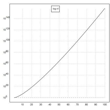
If we want to store all values in a vector, we can use concatenation.
>v=[1]; for i=2 to 8; v=v|(v[i-1]*i); end; v,
[1, 2, 6, 24, 120, 720, 5040, 40320]
Or we can store the results into an existing vector.
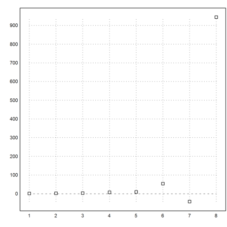
>v=ones(1,100); for i=2 to cols(v); v[i]=v[i-1]*i; end; ...
 plot2d(v,logplot=1); textbox("log n!",x=0.5):
Remember, that loops have to fit into a single command line even if multi-lines are uses.
>A =[0.5,0.2;0.7,0.1]; b=[2;2]; ...
 x=[1;1]; repeat xnew=A.x-b; until all(xnew~=x); x=xnew; end; ...
 x,
     -7.09677
     -7.74194
For such elaborate loops, you should consider EMT programs as shown in the next section.
Of course, the programming language of Euler can also be used to iterate. We give only a few examples here, since the language is described in much detail in a tutorial.
Tutorial about Programs in EMT
For a first example, we define a function to count how long the iteration for the square root takes.
>function map itercount (f$,xstart) ...
 x=xstart;
 count=0;
 repeat
   xnew=f$(x);
   count=count+1;
   until xnew~=x;
   x=xnew;
 end;
 return count;
 endfunction
E.g., we have 5 iterations until the result is good enough, if we start at 2.
>itercount("(x+2/x)/2",2)
5
Since the function vectorizes because of the "map" keyword, we can use it for several start values.
>x=1.5:0.1:10; n=itercount("(x+2/x)/2",x); ...
   plot2d(x,n):
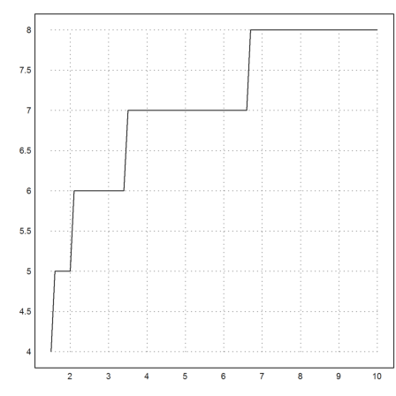
Using the matrix language, we extract the values, where the iteration count increases.
>x[nonzeros(differences(n))]
[1.5, 2, 3.4, 6.6]
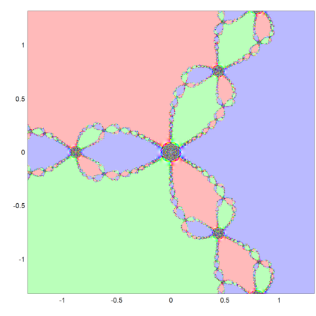
For a second example, we iterate the Newton method of a complex polynomial 10 times for an array of complex numbers.
>p &= x^3-1; expr &= x-p/diff(p,x)
                                   3
                                  x  - 1
                              x - ------
                                      2
                                   3 x
We need a function, which does the iteration 10 times.
>function itertest (f$,x,n=10) ...
 loop 1 to n; x=f$(x); end;
 return x;
 endfunction
Now we can start in a grid of complex values.
>r=1.2; x=linspace(-r,r,501); Z=x+I*x'; W=itertest(expr,Z);
Here are the zeros of this equation.
>z=&solve(p)()
[ -0.5+0.866025i, -0.5-0.866025i, 1+0i ]
To plot, we measure the distance between the 10-th iteration and each of the zeros, and use this to compute a color plot, which shows the limit point for each starting point.
The function plotrgb() uses the current plot window to plot the RGB values as a matrix.
>C=rgb(max(abs(W-z[1]),1),max(abs(W-z[2]),1),max(abs(W-z[3]),1)); ...
   plot2d(none,-r,r,-r,r); plotrgb(C):
To generate a vector of symbolic values in Maxima, there is the function makelist().
>vexpr &= makelist(taylor(exp(x),x,0,k),k,1,3)
                          2           3    2
                         x           x    x
                 [x + 1, -- + x + 1, -- + -- + x + 1]
                         2           6    2
To transfer this to a vector of strings in EMT, use mxm2str(). You can then plot this vector of expressions in EMT.
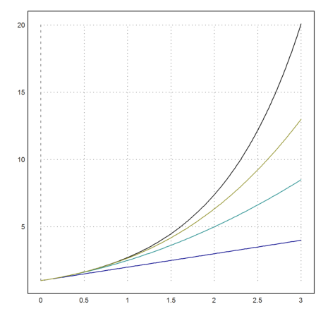
>plot2d("exp(x)",0,3); plot2d(mxm2str("vexpr"),>add,color=4:6):
Of course, you could also extract a single string easily. Then, e.g., plot these expressions in a loop.
>&vexpr[3]
                            3    2
                           x    x
                           -- + -- + x + 1
                           6    2
Maxima does also have a sum() function, which can be used to generate series.
>&sum(sin(k*x)/k,k,1,5)
          sin(5 x)   sin(4 x)   sin(3 x)   sin(2 x)
          -------- + -------- + -------- + -------- + sin(x)
             5          4          3          2
Let us plot
![]()
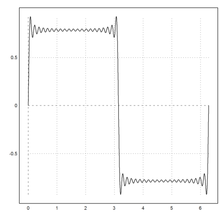
>plot2d(&sum(sin((2*k+1)*x)/(2*k+1),k,0,20),0,2pi):
To achieve the same numerically would not be difficult. Here is an example. We use the matrix language to generate a matrix with
![]()
Then we sum over the rows to get the values of the function at each x[i].
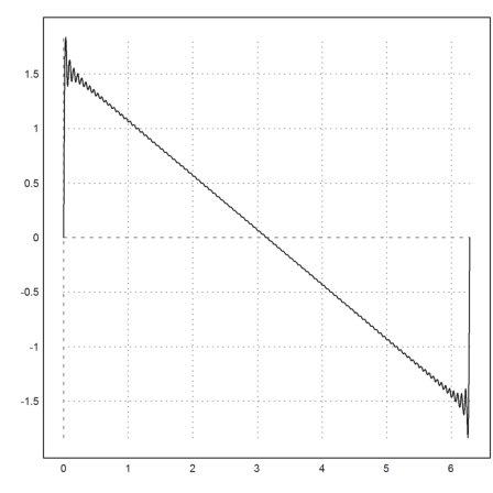
>x=linspace(0,2pi,1000); k=1:100; y=sum(sin(k*x')/k)'; ...
 plot2d(x,y):
There is an interesting way to generate a sequence using Maxima expressions. The mxmtable() command will by default print and plot the sequence, and it returns the sequence as a column vector.
For an example we generate the n-th derivatives of x^x at 1.
>mxmtable("diffat(x^x,x=1,n)","n",1,8,frac=1);
        1
        2
        3
        8
       10
       54
      -42
      944